BIOL 322 Lab 1. Building Population Growth Models in Vensim PLE
When you have completed the exercise below, submit your model and your lab write-up via the Google Drive Form (https://forms.gle/ E3QLACX1aA2Q6ist5). Responses due by the following week's lab period.
During lab, we will work in groups. Here are the groups assigned for today's exercise:
Calvin and Andrea
Emily S. and My
Julia and Shaina
Ricarda and Sophie
Isabel and Merry
Revanth and Elise
Aidan and Amelia
Emily F. and Martha
Diane and Vaughn
Hunter and Kalyan
Overview
For this initial lab exercise, we will introduce the modeling software program Vensim PLE. Before starting this exercise, download and install the free version of Vensim PLE (https://vensim.com/download/) OR you may access the program via the machines in the SCTR A262 computer lab.
IMPORTANT NOTE: These instructions are written for version 9.3.5 of VensimPLE, the version you would download to a personal machine. The computers in A262 use a slightly older version of the program and the icons and menu item names differ somewhat. For help, try this Vensim Quick Reference Guide. Or try the Vensim User Guide, available via the Help menu.
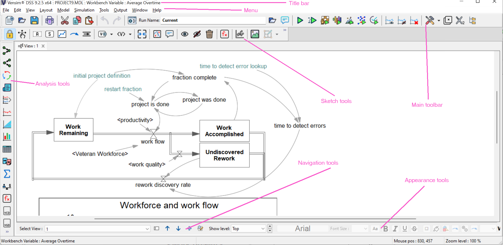
Vensim PLE is a modeling application that allows the construction of a variety of modeling paradigms and the capability of graphical output. On the machine of your choice (your own or the computer lab machine), open the Vensim PLE application. When the program starts up, you should see a window that looks like the image below, without blank space instead of the model in the middle! You may want to download and open this image so you can zoom in to read the labels -- the pink labels are the ones we want to pay attention to. The whole window is the Workbench, with the white space in the middle being where we will construct our models, that's the Build Window.
At the top we have the standard Menu Bar, with the File, Edit, etc menus.
The first horizontal bar of icons is the Main Toolbar, with icon links for things like saving, cutting and pasting, etc.
The second horizontal bar of icons contains the Sketch Tools, which will be important for creating models.
The lefthand vertical bar of icons are Analysis Tools, which will be used for things like making graphs.
At the bottom, we have Navigation and Appearance Tools.
BEFORE WE GO FURTHER, go to Tools --> Options... Click on Toolbars and check the box for Show icon labels. This will give the names below each icon and it will make it much easier to get started.
Learning to Build a Basic Population Growth Model
To get started, we'll build a few simple and familiar models of population growth (which will also form the basis of our later models): the exponential growth model and the logistic growth model. Both of these models describe/predict how the size of a population (number of individuals) will change over time, as a function of other variables like growth rate.
The development of population growth models is motivated by the observation that population size does change in natural populations—in repeatable ways. That is, if you set up an experimental population of organisms, with a renewable food source, you will observe that population size changes (increases) in similar ways in replicate populations (e.g., how quickly population size increases, at what point it stabilizes). This led biologists to fit a function to those lines, which we could then interpret in terms of ecological processes (like births and deaths).
Thus, there is nothing special about the equations that we use here, they were chosen because they fit the observed data reasonably well.
In both models, we assume that individuals are added to the population as a result of births and removed from the population as a result of deaths. We will ignore immigration and emigration for today's models.
Since we know what we want to portray (growth of a population from some starting number, as a result of births and allowing for deaths), we need to think about what variables should be in our model and what should happen to those variables over time.
Population size is the number of individuals in the population. It's the variable we want to recalculate each generation, accounting for births and deaths and record as an output. Usually, we're going to expect it to change over time. We'll need to set a starting value and then check, every generation, to see how it has changed.
Birth rate is how many organisms are born to each organism already present in the population each time step (per capita birth rate). This is the variable that can increase population size. A value of 1.0 means that every individual in your population gives birth to one new individual every generation. Note that we'll imagine for these models that we are counting only females or that our organism is able to clone itself.
Death rate is the variable that can decrease population size (due to natural mortality of individuals). This will be the fraction of the population that dies each generation. So, a value of 0.5 means that half of your population willl die in each generation. Note that logically this variable must have a value between 0 and 1.
Flow equation calculating how to change population size each time step. This is how we will take the information on population size, birth rate, and death rate, to determine how many individuals are in our population in the next time step.
If we think anything else is important in regulating population size, we'll have variables/ components relating to those factors too.
Exponential Population Growth Model
The first population growth model we'll create is the exponential growth model. This is a model in which resources are unlimited so there is no resource-based cap to how many individuals can survive.
How do we graphically represent our growth model? Well, we're going to use a stock-and-flow model, where stocks are ‘boxes' that can count stuff up for us and flows contain the equations that update the value of the stocks based on other parameters that we specify (like birth or death rate). So in our model, population size will be a stock and the equation calculating change in population size will be a flow. The stock and flow will be connected so that the flow can change the value of the stock each timestep.
Before we actually construct the model, let's look a little closer at the math we'll be thinking about to create this model. If we consider a population of organisms, newborn organisms arrive due to births and other organisms depart due to deaths. In VensimPLE, we can represent births as a flow IN and deaths as a flow OUT. Or, we can use a single bidirectional flow, where the overall direction of the flow (increasing or decreasing the stock's value) is the net result of birth rate minus death rate (b − d). Thus, growth rate is r = b − d, the intrinsic rate of increase. Note that r usually represents the maximum rate of growth. We will model the size of the population over time based on the rate of birth (b), the rate of death (d), and the current value of N (population size). Right now, we're not worrying about genetics-—as if we are assuming everyone is the same genotype—-so we aren't tracking different genotypes, just counting the number of total individuals.
So, if we have population size at time zero, N0, and we want to know population size after one time step, N1 (one generation), we are going to use the exponential growth equation:
In the two-flows model, remember that we'll have to separate the calculation for birth and the one for death into two different flows. But in the single flow version, we'll have a flow for growth which will contain the equation N*(b-d). Let's get started on the two flow exponential model.
Two-flow exponential model
To start, find and open the Vensim PLE program (either look in the Applications/Programs folder or use the Search function). Once the program opens, click the New Model icon, which will open up a Model Settings window. We want to use the following values for Model Settings:
Units for Time
Year
INIITIAL TIME =
0
FINAL TIME =
100
Time Step
1
Now, before we do anything else, save your model! Call it twoflow-exponential. And make sure to save as you go along just in case something crazy happens.
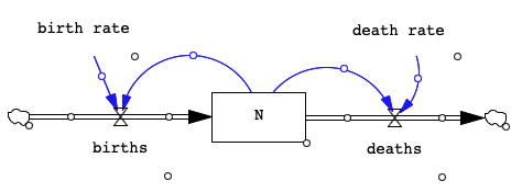
To create our model, we will first add all of the components of the model onto the Build Window (the big white space). That will be a stock for population size (called N), a flow for births, a flow for deaths, a birth rate (b), and a death rate (d).
To add a stock component to the model canvas (to represent population size), click on the Stock icon (S in a box) in the second horizontal (top) icon bar. Then click somewhere in the white area, the Build Window. In the box that pops up, type N the variable representing population size.
Next we'll add the births flow and the deaths flow. Click on the Flow icon (arrow in a tube) on the second horizontal menu bar and then click in the space to the left of your N stock. Now move the cursor over the box representing the stock N and click on the box representing N. You should see an arrow appear, pointing toward stock N. Name it births. Note that the cloud on the left just represents somewhere else, unaccounted for in the model from which things come. It does not have to be connected to anything. But the arrowhead must be connected to our stock.
Now add the deaths flow. You may be able to do this without clicking on the Flow icon again. Click on the stock N and then click a second time about an inch to the right of the box. You should see a new flow appear, the arrow pointing OUT of the stock N. Name this one deaths.
As you may guess, flows add things into the object they point toward and take things away from objects they point out of. So the value that goes into deaths will be subtracted from N while the value in births will be added to it.
Next, we can add the rate variables, birth rate and death rate. For birth rate, click on the Variable icon (a box with an A inside) and then click on the Build Window, a little above the births flow. Name this variable birth rate. Repeat this procedure for death rate, placing it above the deaths flow. When you are finished, click on the Move icon to avoid adding more variables to the Build Window.
Finally, we can add arrows telling Vensim which variables can be used in equations for other variables. In this model, that means we need to connect other variables to the flows since those will have the equations in them. Click on the Arrow icon on the second horizontal bar, then click on birth rate, move your cursor over the births flow and click on the births flow. You should see a pink arrow going from birth rate to births. Do the same to create an arrow from N to births. Lastly, create an arrow from death rate to deaths and from N to deaths.
Note that you can change the shape of arrows by dragging the circle in the middle of the arrow shaft. You can also position arrows by clicking on white space in between the two endpoints, as you are setting up the arrow. If you want to delete a component, click on Delete and then click on the component you want to remove.
Your model should now look something like the following. Notice that stocks are in boxes, flows have this hourglass and arrow structure and other variables (rates or constants) have no surrounding shape. All components have a small circle in the bottom right corner, this is used for moving and resizing.
Now we've created the image of the variables we want to include, we need to give them values so the model will know how they are related to each other. We will choose an initial population size and after the first time step, the pop size will be determined by the values of the two flows. We'll put equations in the flows, using the existing population size and the birth or death rates (which give us how many babies per current individual or how many deaths of the current individuals). The birth and death rates can be constant values or we can set them up to vary. We'll start by making them constants.
To add values or equations to our variables, we click on the Equation icon on the second horizontal bar (fx inside a box). All of the variables in our model will be highlighted since none of them have equations in them yet! Now we will click on them one at a time and set the correct parameters.
Let's start with the population size, N. Click on the stock N and a box will pop up with lots of options. Under Equations, you will see that births minus deaths is already entered, the program assumed this based on how we set up the flows. But at the moment there are no organisms in our population, so we need to set the Initial Value to be 10. For now, that's all we'll change, everything else should be fine. Click Ok to accept the change you made and close the pop up.
Next up, click on birth rate and in the Equations box, type 0.3. Now just above the Equations box, set Min to 0, Max to 4 and Incr to 0.1 (that's increment, how much you can change it by at a time).
For death rate, set Equations to 0.2, Min to 0, Max to 1.0, and Incr to 0.1.
Now to set up the flows. Click on births. In the Equations box, type birth rate * N. You can type it or you can click on the variable names in the box to the right and below. Only the variables connected by arrows in are allowed to be used. For the deaths flow, enter the equation death rate * N and click Ok.
It's time to run our model and see what happens to population size if we start with 10 individuals and then have birth rate of 0.3 and death rate of 0.2 (you can hopefully guess what will happen...). To run the model, click on the Simulate icon (a green play button). A small pop up will quickly appear and disappear but we don't see the results until we create a graph.
To create a graph, click on the variable you want to graph, N. Because this is a model of change over time, we know that the x-axis will be time (in years) and the y-axis will be our variable of interest, N. After clicking on N, then click on the Graph icon on the left hand icon bar. A graph should pop up showing exponential growth!
Now, remember how we put in those min, max, and increment values for birth rate and death rate? Here is where we can use that info! Click on the SyntheSim icon (next to the Simulate icon). You should see sliding bars pop up for birth rate and death rate and small graphs appear below births, N, and deaths. These graphs show the updated results of the model if you slide the button for birth rate or death rate. Try it out, change the birth rate to 0.1 instead of 0.3. When you are finished testing it out, click the SyntheSim exit button (x in a hexagon). If you want to get a larger graph with a change birth rate or death rate, you will need to go back in to edit the equations for those variables, then click Simulate again.
When looking at graphs, you should pay attention to things like how long it takes to reach equilibrium, if such is reached. In the case of the exponential model (which does not stabilize), you might notice things like how long it takes for the population to reach a size of 100. Remember we are thinking of the time axis as representing generations in a population.
Graphs will often be the thing we want to retain to show us what's happening. To save your graph, go to File -> Save. You can zoom in or out or adjust the scale (say select only part of the x-axis) by clicking on the graph. Reset using the View menu, Reset Scale.
Single flow exponential model
Now, you are going to build the same model that you just did with one difference: instead of using a flow in and a flow out, you are going to use a single flow that adjusts for both births and deaths at the same time. We'll still have the birth rate and death rate, we'll just use the equation for dN/dt that we saw above, where r = b - d. You could call the new flow 'popgrowth'.
You could build this model in the same Build Window though you'll have to name the variables differently if you do (you could add a 1 to each variable name). Alternatively, you can just open a new model, File → New. Save it with a descriptive name, like “singleflowexponential”.
Build this one without my step-by-step instructions so you can practice using VensimPLE. Make sure your model gives the expected output in the graph! (It should be just like your two-flow model.)
Logistic Growth Model
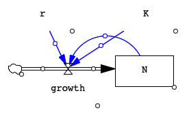
Next, you are going to build a model of population growth when resources are limited but renewable — the logistic growth model. In logistic growth models, we assume that the renewable resources available in the environment can only support so many individuals and thus the rate of growth varies depending on the density of the population, slowing down as the population approaches the carrying capacity. At carrying capacity the rate of growth will be zero since no more individuals can be supported. The equation for logistic growth is:
dN/dt = ΔN = rNt(1 - Nt/K)
This model includes the parameter K, the carrying capacity of the population. In this model, we usually use r to represent the maximum rate of growth and we don't separate the effects of births and deaths. You can think of r(1 − Nt/K) as the actual rate of growth, given the population K density.
With your group, go ahead and try to build this model (see image below). Note: Do not use the equations from the exponential growth model when building the logistic model. However, you can use r instead of having separate values of b and d.
When you set up the model, you will have similar parameters to your exponential model but you will also have a carrying capacity (K). Let's use K = 200, r = 0.3, and set initial N to 10 like we had earlier.
Once you get your model running, let's explore what happens when you change the value of r. With K = 200, we'll try r = 0.3, r = 1.0, r = 2.0, r = 2.5, r = 2.7. Instead of using SyntheSim like we did earlier, we're going to learn another way to test out different conditions: using Simulation Control.
Click Simulation Control on the first horizontal icon bar. A box will pop up where we'll save the changes we make. In the popup box, change the run name to r0p3 (you can't use decimals in the run name) and in the Comment box type 'r = 0.3', this will be our default run where we don't change the value of r. You can click on r to confirm it is set to 0.3. Click Save Changes and then click Simulate.
Now we want to create a new simulation with r = 1.0. Click on Simulation Control again and this time change the run name to r1p0 and in Comments type 'r = 1.0'. Click on the variable r and change the value to 1. Then click Save Changes and Simulate.
Repeat those steps with the appropriate alterations to create simulations for r = 2, r = 2.5, and r = 2.7.
Once you have created all the variations, click Simulate on the horizontal menu bar, click on N, and then click Graph. A graph should appear that has a line for each value of r that you tested. You can unclick them from the legend to declutter the graph and figure out what's going on. Start with just r = 0.3 and then add the higher values one at a time. What happens? How might we explain what's going on? (Think in terms of biology.)
What's Next?
If you want, go ahead and explore more of the features of VensimPLE. For example, you can use Comments to leave notes for yourself (or me) on the Build Window. Or maybe to record info that you will need later.
Lab Write-Up
For this lab exercise, you gained some experience using the program VensimPLE to build simple population growth models. As a write-up please respond individually, in narrative form, to the following questions:
Imagine a friend asked you what you did in lab today and provide a brief description.
Was anything confusing or interesting to you about using VensimPLE and building the models?
Describe how population growth differed between the exponential and the logistic models. What happened when you varied the value of r in the logistic model? What do you think is going on? Hint: think about what the large values of r mean.