BIOL 322 Lab 3. Genetic Drift

When you have completed the exercise below, submit your model and your lab write-up via the Google Drive Form (https://forms.gle/ E3QLACX1aA2Q6ist5). Responses due by the following week's lab period.

During lab, we will work in groups. Here are the groups assigned for today's exercise:

Overview

Today, we'll create a modified version of our Hardy-Weinberg model from last week and we'll add genetic drift. Think about how we describe the effects of genetic drift on genetic variation. Starting with our base HW model, which parameters should we adjust and what things do we need to add to incorporate genetic drift?

This is somewhat complicated, since drift is a stochastic process. Remember from Chapter 6, we know the variance in allele frequency change due to drift; we can use that to add drift to our gene pool. "Drift" will be a change to the allele frequency, where the value will be a random number chosen from a normal distribution with a mean of zero and the binomial standard deviation. In this way, we add (or subtract) a small, random number to the allele frequency each generation. We'll make this change and then use the adjusted allele frequency (padj) to randomly combine alleles to form zygotes.

Note that this should mean our population will always remain in HW proportions, even though allele frequencies will be changing each generation! This is a good demonstration of the fact that nonrandom mating is the only thing that puts a population out of HW proportions. For other evolutionary forces, we must examine change in allele frequency across generations to detect the effects.

Building the Drift Model

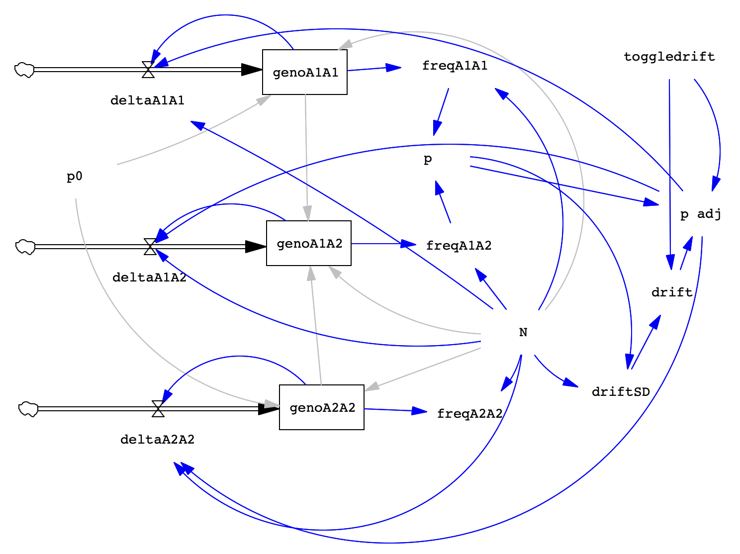
To begin, we'll set up a model similar to the HW one, except we'll only keep track of 1 allele (which makes it easier to add the stochasticity to the model without messing things up!). Here's a screenshot of the final product, for reference as we proceed:

1. Open a new model and input the following settings:

Units for Time	Year
INIITIAL TIME =	0
FINAL TIME =	1000
Time Step	1



2. Create a stock for each genotype, perhaps named: genoA1A1, genoA1A2, genoA2A2. Like in the image, be sure to leave space for the additional variables we'll be adding!


3. Next, add the flows, one per genotype stock. Be sure that the arrow on the flow connects to the stock. We name these delta11, deltaA1A1, deltaA1A2, deltaA2A2.


4. Now we have a number of additional variables to add:

Variable	Description
N	population size, which we'll want to manipulate with Simulation Control
p0	this is the starting frequency of the A1 allele, we'll also vary this with Simulation Control
freqA1A1	the observed frequency of the A1A1 genotype
freqA1A2	the observed frequency of the A1A2 genotype
freqA2A2	the observed frequency of the A2A2 genotype
p	this is the frequency of the p allele, measured every generation, this is the primary variable we are interested in tracking to determine effects of other variables on it
driftSD	the standard deviation for the distribution of changes due to drift; this will vary depending on the population size and is used in the drift variable
drift	the actual amount by which we will change the value of p for the next generation, causing change due to drift
p adj	the adjusted value of p, so the new value of p after adding the effect of drift; this is what we use to create the next generation
toggledrift	this variable let's us run the model with or without causing drift to happen; you adjust it once per run, drift is either on or off for the whole simulation, makes it easy to see what the effect of drift is compared to HW equilibrium



5. Next, you need to add the appropriate arrows, try to follow the image above. You can check the Arrows Key table if needed (see the drop-down menu).
   
6. Once we have our arrows placed, we are now in position to enter the equations for each variable. If we don't have the arrows correct, we won't be able to put the right equations in, so pay careful attention.


7. Remember, to enter equations, click on the Equations icon and then click on the variable whose info you want to edit. In the box that pops up, you enter the correct information for that variable. We have a lot of variables so let's take this slowly.


8. Let's start with the variables that we are just setting a value to initiate the model. For these, the equation is simple, it's just the starting value we are choosing to use. Use the following equations for the varibles below:

Variable	Parameter	Value	Min	Max	Incr
p0	Equations	0.5	0	1	0.01
N	Equations	100	0	500,000	1



9. Having set up N and p0, we can enter the initial values for the genotypes. Since we are assuming that mating is random, we expect genotypes to occur according to HW proportions, so we'll use those equations to set the initial value for our genotypes, multiplying by N so we get the number of individuals, not just the frequency.
   • Make sure you do NOT change the equation entry for the genotypes, that is already set up correctly to be the value of the flow.
   
   
   • Click on 'genotypeA1A1'. What should you enter for the initial value? (p0 * p0 * N)
   
   
   • For genotypeA1A2, use the equation N - genoA1A1 - genoA2A2. That ensures that we end up with the right number of total individuals, N.
   
   
10. Once we have the numbers for the genotype stocks, we can set up the equations for freq11, freq12 and freq22. We mainly want these variables for ease of graphing and manipulation to do other calculations. What should the equations for these variables be?
• Example: freq11's equation is geno11 / N


11. Now to the variable of greatest interest: p! How do we calculate the frequency of the allele using the genotype frequencies? If you aren't sure, check with Angie. You can also check the key at the end though it's best if you can try to work it out.


12. For the variables related to drift (driftSD, seed, drift, and toggledrift and p adj), the equations are somewhat complicated so we'll learn a little about how they work as we enter them into the model. Also see the table below for quick reference.


• driftSD is the standard deviation for the amount of change due to drift. Since change due to drift is random, it could be a positive value or a negative value but we know the amount of change depends on the population size. In a small population, a large change is more likely to occur than in a large population. We can control this factor with the variable driftSD. We're using the equation for binomial variance here, you will see that how likely small versus large changes are depends on the current allele frequency and the population size. The square root part occurs because the standard deviation is the square root of a variance.
  
  The equation is: SQRT( (p * (1 - p) ) / (2 * N) )


• toggledrift is the variable we will use to turn drift on or off and to tell Vensim to create a new simulation run with drift (we will use it as a seed in the equation for drift). This is useful so that we know what would happen if drift was not occurring and also to allow us to check that the model is set up correctly. It will also help us to run multiple replicate runs in which drift can act differently -- each different value of toggledrift will correspond to a different random outcome of the model. The value of toggledrift = 0 will be special though, that will be what we use to run the model with no randomness at all. We will encode this ability when we put in the equation for p adj, which we'll do shortly. Here's the equation and other values to use:



Variable	Equation	Min	Max	Incr
toggledrift	0	0	10000	1



• drift is the variable we'll use to figure out (randomly) how much p changes by chance, calculated anew each generation. We just set up the standard deviation (SD) for this distribution, now we use a function (RANDOM NORMAL) to choose a value from the distribution. Change is equally likely to be an increase as a decrease, so we'll use a mean of zero. For this function, we also have to specify a minimum and a maximum so we'll use -1 and 1 since allele frequency can't possibly be larger or smaller than that! The function requires arguments in the following order RANDOM NORMAL(min, max, mean, sd, seed)
  
  The equation is RANDOM NORMAL(-2, 2, 0, driftSD, toggledrift)


• We're finally ready for the most complicated equation of all, the one for adjusting the allele frequency for the effect of drift, p adj (p-adjust). For this variable, since we want to turn drift on and off, we need to use an if statement -- what to do when drift is on and what to do when it's off. We also need to make sure that when we add together p and drift, we don't get a value less than zero or greater than 1. If so, we just want the value to be 0 or 1, since it's impossible in reality to exceed these limits. The function in Vensim that we need is IF THEN ELSE( _cond_ , _ontrue_ , _onfalse_ ). You can see it requires 3 arguments (the if condition, what to do when it's true, and what to do when it's false). We actually have 3 if conditions to meet so we're going to have a complicated nested if-then-else statement. Here's the equation and I'll provide a text explanation after it.
  
  IF THEN ELSE(toggledrift=0, p , IF THEN ELSE( (p+drift) >= 1.0 , 1 , IF THEN ELSE( (p+drift)<=0 , 0 , p+drift ) ) )
  
  You can see the three if-then-else functions. Reading this from left to right, this statement says IF toggledrift is set to be 0, then make p adj be the same as p (this is what happens when there is no drift). But the ELSE part says, IF (p + drift) is greater than or equal to 1.0, make p adj equal to 1.0 (this ensures we don't have more than 100% A1 alleles, which is impossible). And then the second ELSE says IF (p + drift) is less than or equal to zero, set p adj to be 0 (preventing us from having negative numbers of alleles). Finally, the last ELSE says if none of the preceding things are true (thus, p + drift is between 0 and 1), set p adj equal to (p + drift).


13. Ok, that was the hardest part. All we have left are the equations for deltaA1A1, deltaA1A2, and deltaA2A2. Because we are causing drift to happen on allele frequency directly, these equations will be similar to what we used last week with the HW model, just using p adj instead of p. So, for deltaA1A1, we get:
    
    deltaA1A1 equation is: (N * p adj * p adj) - genoA1A1
    
    Go ahead and set up the equations for deltaA1A2 and deltaA2A2 as well.


14. Once you have finished entering equations, check to make sure they are correct (you may want to use the key at the end). Then we are ready to click Simulate to run the model. To get a graph, select the three genotype stocks (or whatever variable you want) and then click Graph. Remember that we set up the initial conditions so that drift will NOT occur (toggledrift = 0) so we expect to see just the HW model.
    • What happened? Does anything change on the graphs? What did you expect to see? Consider your responses as you write up the lab exercise in the next section.
    
    
15. Now, to make sure that drift can occur as expected, we need to use Simulation Control to alter the value of toggledrift and then Simulate the model again.


• Click Simulation Control on the first horizontal icon bar. A box will pop up where we'll save the changes we make. In the popup box, change the run name to nodrift and in the Comment box type 'toggledrift = 0', this will be our first run where we don't change the value of toggledrift. Click Save Changes and then click Simulate.


• Now we want to create a new simulation with toggledrift = 1.0 so that drift will occur. Click on Simulation Control again and this time change the run name to run1 and in Comments type 'toggledrift = 1'. Click on the variable toggledrift and change the value to 1. Then click Save Changes and Simulate.


• Let's make one more simulation with drift. Click on Simulation Control and name this one run2, in Comments: toggledrift = 2, and finally click on toggledrift and change the value to 2. Click Save Changes and then Simulate.


16. Once you have created those variations, click Simulate on the horizontal menu bar, click on p, and then click Graph. A graph should appear that has a line for each value of toggledrift that you tested. What happened? How might we explain what's going on?
    
    Note that for the drift model, we are primarily interested in what happens to the allele frequency, p, over time. So instead of graphing genotype frequencies, we want to graph allele frequency. We could also graph heterozygosity, as that's our common estimate of genetic variation.
    
    (Sidebar: you should see a flat line for the nodrift run and then two squiggly lines that are different from each other for run1 and run2.)

Lab Write-Up

Now that you have created an awesome working drift model, let's see what happens with multiple runs and altering starting conditions. Remember that since drift is a stochastic process, we cannot predict the outcome of any particular run but we can see trends from multiple runs. Thus, we'll need to look at multiple runs of any conditions we are testing out to identify trends. Remember that the effect of drift depends on both initial allele frequencies and total population size (a larger population takes longer to reach equilibrium).

For the questions below, you should pay attention to the following values for each run so that you can compare across different runs. Which variables change the outcome and in what ways? Does the time to fixation change? Does the size of change from one generation to the next change?

• population size
• length of run (how many time steps before p = 0 or 1; time to allele extinction or fixation)
• where allele frequency started and where it ended up (graph p)
• where heterozygosity started and where it ended up (graph freqA1A2 to see this)

So you will be graphing p and possibly freqA1A2 (heterozygosity).

Examine the trends associated with these variables when you run the scenarios below. Before running them, try to predict what you think will happen and which variables will matter the most. Consider how the differences between scenarios demonstrates the way in which drift influences genetic diversity.

Questions

1. Explore the effect of initial allele frequency on the outcome of the runs. Do 10 runs for each of the following sets of starting conditions:

   Trial	p0	N	Final Time	toggledrift	# runs
   1a	0.5	100	1000	1 to 10	10
   1b	0.2	100	1000	1 to 10	10
   1c	0.8	100	1000	1 to 10	10

   
   The easiest way to do this is to change the default values for p0, N, and Final Time then use Simulation Control to just change the value of toggledrift 10 times. You want 1 graph of p showing all 10 runs of trial 1a, a separate graph of the run for trial 1b and for trial 1c. You can change the Final Time by clicking on the Model drop-down menu and choosing Settings... I also suggest saving your graph for each trial. To save a graph, go to File --> Save. You can also rescale and zoom in or out by clicking on the graph (use the View menu to reset the scale).
   
   Now, tell me what you notice about what happens in these runs. Is equilibrium reached? Fixation or extinction? What changes when you change starting allele frequency? Write a summary of your observations.


2. Examine what happens when you change population size. Use the following sets of starting conditions:

   Trial	p0	N	Final Time	toggledrift	# runs
   2a	0.3	10	1000	1 to 10	10
   2b	0.3	100	1000	1 to 10	10
   2c	0.3	1000	1000	1 to 10	10

   
   Again, you should do at least 10 runs for each value of population size so that you can try to detect any trends. What trends do you notice? How does population size influence the equilibrium that's reached? Feel free to explore what happens with other values of N or with other values for p0. Write up a summary of your observations.


3. Finally, in paragraph form, give me a summary of the overall ideas/patterns demonstrated in the drift model (you don't need to repeat yourself from earlier questions). Reflect on what you've observed. Are any of the results surprising to you? Or do they change how you think about the consequences of drift? How might these results influence thinking about drift as a potential issue in conservation? (You are, of course, welcome to test out other conditions in your model!)

Remember to submit your model and responses as a PDF via the Google Drive Form: https://forms.gle/E3QLACX1aA2Q6ist5. Write-up are due by the next lab period.

Key to Arrows

Below find the key to arrow placements for each variable.

Key to Equations

Below find the table of equations for each variable.