Manual
Part A.3. Creating Dendrites
A.3.a Creating Dentritic Processes
IN section A.1 , we defined our final product to be a model of a network of subthalamic nucleus projection s. Since then we have created a soma with passive channels, Hodgkin and Huxley channels (membrane mechanisms) and an electrode (a point process). However, we have no dendrites.
In this tutorial, we will add dendrites to the previous model SomaGUI.hoc. As part of adding dendrites we will learn:
- how to create additional sections (dendrites)
- how to connect them to different sides of the soma we've already created
We recommend that you open SomaGUI.hoc in a text editor and save it as CellGUI.hoc. As in previous tutorial, type the code that is highlighted into the file. Remember to save it periodically. Save it in the same folder as SomaGUI.hoc.
A.3.a Creating Dendrites
Before we do anything be sure the following code is in your CellGUI.hoc text file:
load_file("nrngui.hoc")
create soma
access soma
soma nseg = 1
soma diam = 18.8
soma L = 18.8
soma Ra = 123.0
soma insert hh
soma insert pas
objectvar electrode
electrode = new IClamp(0.5)
electrode.del = 100
electrode.dur = 100
electrode.amp = 0.45
print soma.v
forall psection()
tstop = 300
As was described in the A.1l, works with cylindrical sections. So far, we have only created a single section containing a single compartment representing the soma. We are now going to add more sections representing the two dendrites. These can be created just as the soma was created. To do so modify the create line in the program accordingly:
create soma, dend[2]
Each section listed after the create command is separated by a comma. In the case of the dendrites, we use an array to represent the two dendrites. We could have created two different sections named dend1 and dend2, but, as you will see below, representing sections (and objects) as arrays has many benefits. The array indices are numbered from zero, so to access the first element of the array of dendrites, you need to use dend[0], and to access the second element, you need to use dend[1]. If arrays are unfamiliar, you can read about them in most programming books.
One small note on programming style: In the future, if we want to re-use this code for another that contain, for example, 4 dendritic trunks, we will have to change all of the 2's to 4's in the code. We can avoid this by using a variable to represent the number of dendrites. We need to create and reference the maximum number of dendrites through this variable throughout the program. For example:
ndend = 2create soma, dend[ndend]
access soma
This will give us the same result as above, but now if we want to re-use this code in the future to represent 4 dendrites, all we have to do is change ndend from 2 to 4.
We have a good anatomical description of the subthalamic nucleus projection dendritic tree (obtained from experimental data):

For simplicity and ease of computation, these two dendritic trees can be reduced to single equivalent cylinders (see Rall and Agmon-Snir, 1998, for the requirements and procedure). We will explore methods for constructing full dendritic trees in the tutorial titled "Creating realistic morphology". Collapsing the trees produces the following visual description of our subthalmaic cell:

Segments within a section
We could create one of our dendrites using the following hoc code:
dend[0] {
    nseg = 1
    diam = 3.18
    L = 701.9
    Ra = 123
    insert pas
}
This syntax for defining the properties was described as Method 2 in the first tutorial. The code could alternatively be written as was done for the soma but as you'll see later, this formulation has it's advantages.
Each of the equivalent tree cylinders is very long, so this definition of a dendritic section has the disadvantage of only having one compartment. What this does is make the entire equivalent dendritic tree behave as if it were a single point -- without any spatial differences. Normally we think of electrical potentials travelling down the dendrites to the soma implying that spatial dimensions are important. To increase the spatial resolution of the dendrite, we can simply increase the number of segments in the section. In cable theory terms, this has the effect of increasing the spatial resolution of the cable equation. This is very important for accurate simulations. If the section's number of segments is too small, then the spatial resolution is low and you might not be able to see the fine details in the simulation results. If the section's number of segments is too large, then you might be unnecessarily extending the simulation time. By analysing the effects of spatial resolution on the results (in addition to other analyses), you can achieve efficient and accurate simulation results.
The reason for 's distinction between sections (high level conceptual modelling construct) and segments (low level numerical simulation detail) is to allow you to create models that do not rely on the number of segments (or compartments) in the model. Rather, you can create a model entirely independent of the numerical details. Then, if during the analysis you find you need to increase the spatial resolution in a certain part of the model, you can do so simply by increasing nseg for that section.
For our simulation, we are interested in seeing the potentials travel along the dendrites, so we want to increase the number of segments. Therefore we give each of the two dendrites five segments each:
Insert this text into the .hoc document after "insert hh insert pas":
dend[0] {nseg = 5 diam = 3.18 L = 701.9 Ra = 123 insert pas}
dend[1] {nseg = 5 diam = 2.0 L = 549.1 Ra = 123  insert pas}
Now that we have all of the sections created and their properties set, we need to connect them together.
A.3.b Connecting the dendrites to the soma
Since uses the abstraction of sections (instead of specifying individual compartments), we need a way to refer to specific points along the section. This is handled by using the section name followed by a number between 0 and 1 in parenthesis which represents the distance along the section. For example, dend[0](0) refers to a point at the proximal end of dendrite 0, dend[0](1) refers to a point at the distal end of dendrite 0, and dend[0](0.2) refers to a point 20% down dendrite 0:

We use this notation when connecting sections to one another since we need to specify what point of one section connects to what point on another section. We also use this notation when we place point processes in a section.
This method of specifying a point on the section is conceptually independent of the number of segments in the section. Thus, when you insert a point process (as in the current stimulus in A.1 ) 50% down the section, it is physically inserted into the segment that contains the point 20% down the section.
However, due to the way works, if you later change the spatial resolution of the section, the point process may no longer be in the segment containing the point 20% down the section. The moral is that it's best to specify nseg before attaching point processes. The box contains a more detailed explanation of this point.
Expert tip 1: Why it's better to specify nseg before attaching point processes
Suppose nseg is 1 and you try to put an IClamp at 0.1, as in this cartoon.
It will actually end up at 0.5, as shown here. This is because the segment is one electrical compartment, so it doesn't make any difference to the simulation where the electrode is placed. allocates the position to be the centre of the segment rather than keeping track of where we wanted it placed.
Later, you decide to increase nseg to 3. What happens to the IClamp? It stays put at 0.5, right in the middle of the second segment, even though the first segment is the one that contains location 0.1.
So it's best to specify nseg before attaching point processes.
Expert tip 2: How to move point processes after changing nseg
If you do have to increase nseg after placing point processes, you can re-position the point processes in order to take full advantage of the improved resolution. For example, if our current clamp was called stim, we could move stim to 0.1 with the hoc statement stim.loc(0.1) and the result would be as shown here, i.e. much closer to 0.1 than if we had left it at 0.5.
For our simulation, we are going to connect the soma and the dendrites together. We use the connect command to accomplish this:
connect dend[0](0), soma(0)
connect dend[1](0), soma(1)
Our entire full morphology subthalamic code now contain the following code:
load_file("nrngui.hoc")
ndend = 2
create soma, dend[ndend]
access soma
soma nseg=1
soma diam=18.8
soma L = 18.8
soma Ra=123.0
insert hh
insert pas
dend[0] {
nseg = 5
diam = 3.18
L = 701.9
Ra = 123
insert pas
}
dend[1] {
nseg = 5
diam = 2.0
L = 549.1
Ra = 123
insert pas
}
// Connect things together
connect dend[0](0), soma(0)
connect dend[1](0), soma(1)
// create an electrode in the soma
objectvar electrode
soma electrode = new IClamp(0.5)
soma electrode.del=100
soma electrode.dur=100
soma electrode.amp = 0.45
print soma.v
tstop = 300
forall psection()
Notice the use of // in the supplied sample code. Anything after the double forward slash is considered a comment, so it is a useful way of explaining your code. Since our code is becoming more complex, it makes sense to set various parts apart using spaces and comments.
Note on initialisation.
The initial value of the membrane potential (v_init; as seen in the RunControl window) will be close to the resting potential in each compartment, but not necessarily the same. It will generally take a few milliseconds for the membrane potential v to settle down the the "correct" value in each compartment. This isn't just because v_init isn't "correct"; if a model has significant electrotonic extent and the spatial distribution of channels is nonuniform, the steady state membrane potential will in general be nonuniform.
To avoid this transient phase, it's a good idea to let the simulation run for a while before performing the experimental manipulations. In the example above, we wait 100 ms before injecting current. (This delay appears in the code as .del = 100)
(You can see this voltage wobble in a voltage axis. The state variables, in particular the inactivation variable h_hh, also take a while to settle down; we will learn later how to look at them.)
Save and run the program by double clicking on the file in the folder. Your display should consist of the Main Menu window and the terminal window. In the terminal window you should see the properties of not only the soma but of 2 dendrites, dend[0] and dend[1].
A.3.c. More graphs
Before we plotted the voltage change as recorded in the soma section of our program. It was the default section and it was the only section. Now we have 3 sections and essentially 11 segments from which we could record.
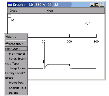
It would be useful to compare the voltage of the soma and a distal part of a dendrite on the same graph (in different colours). To do so open a voltage graph (Graphs>>Voltage axis). You will see the legend "v(.5)". This means we are plotting the voltage halfway down the default section (the section defined in the access command - in our case the soma).
 In order to access
the graph properties, including, for example, adding a
dendritic voltage plot to the graph, right
click on the voltage axis. This brings up a Graph
Properties menu. Chose Plot what?.
This should bring up a window from which we can choose a variable to plot. The variables can be either directly typed in if we know the exact name of the variable we want to plot, or they can be selected from the list of variables in the selection boxes.
We want to plot the voltage from a distal dendrite, so we need to select dend[0] in the first selection box (double click on the text) and then select v(0.1) from the second box (again double click on the text). You can change the position from which the recording will be made by changing v(0.1) to v(0.9). This modification will make a recording at the more distal end of the dendrite.
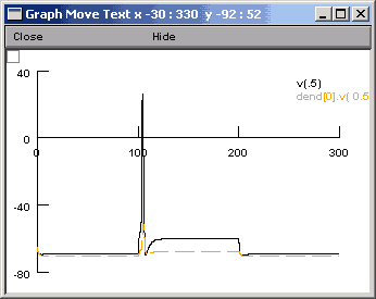
Finally, we press the Accept button. The legend dend[0].v(0.9) will appear on the voltage axis. Now when we run the simulation, we will see two traces. However, it would be nice if they were different colours. To change the color and thickness of the lines we can select Colour/brush from the Graph Properties menu (after right clicking on the graph). This brings up a palette of colours and lines.
We select color and/or line types by clicking the button in front of the color or line type and then clicking on the relevant legend. After we have run the simulation again, we should see something like this:

Be careful in that clicking on the legend of the other line will cause the other line to also turn red. Before doing too much damage, it might make sense to right click and select "Move text" or another command. In this way you will not accidentally change the color of the lines.
Besides voltage axes, there are several different axes available when plotting variables vs. time (Voltage axis, Current axis and State axis). Each of these require their own graph since the method used to solve the cable equations, developed by Mike Hines, calculates each of these variables at different times. For example, voltages are calculated at each time step, but currents are calculated at the half time step before voltage and the state variables are calculated at the half time step after the voltage. For more information on the numerical method used to solve these equations see Hines (1984).
The principles of using the other types of axis are the same as using the voltage axis. To confirm this, try using current and state axes to display currents and the state variables at different points on the .
SUMMARY
- Created dendrites (using variables to define multiple dendrites)
- Connected the dendrites to the soma
- More on graphing (voltage graphs)
Next: Part B: Creating more realism - Subthalamic s
References
Rall, W. and Agmon-Snir, H. (1998) "Cable theory for dendritic s" in Koch, C. and Segev, I., editors (1998). Methods in al Modelling: From Ions to Networks. MIT Press, Cambridge, Massachusetts, second edition.
Hines, M. (1984) Efficient computation of branched nerve equations. Intl. J. Bio-Med. Comput. 15:69-76
Acknowledgements
Last modified on 10/29/04 by
Albert Borroni, CS/Neuoriscience Oberlin College (aborroni@oberlin.edu)
based on tutorial written by
Andrew Gillies (andrew@anc.ed.ac.uk)
David Sterratt (dcs@anc.ed.ac.uk)
which is originally based on the tutorials by Kevin E. Martin
with the assistance of Ted Carnevale and Michael Hines
After creating the soma and dendrite sections, we need to set their properties and add the appropriate channels. We've done this already for the soma but for this exercise we will use method 2 to set the properties of the soma. Method 2 uses a curly brackets to group all the parameters associated with a particular section. Replace the different lines referring to the soma section's properties in CellGUI.hoc with the following code:
soma {
    nseg = 1
    diam = 18.8
    L = 18.8
    Ra = 123.0
    insert hh
    insert pas
}
The above code will set the number of segments, the diameter and length of the soma as well as insert Hodgkin-Huxley channels.
Acknowledgements
Last modified on 10/29/04 by
Albert Borroni, CS/Neuoriscience Oberlin College (aborroni@oberlin.edu)
based on tutorial written by
Andrew Gillies (andrew@anc.ed.ac.uk)
David Sterratt (dcs@anc.ed.ac.uk)
which is originally based on the tutorials by Kevin E. Martin
with the assistance of Ted Carnevale and Michael Hines