Manual
C.3 Graphing with the GUI
Using the code (SubThalNucl2.hoc) developed in the previous tutorial, this tutorial will show how to visualize the many s in the Graph>Shape plot window, how to manipulate voltage axis graphs and how to save a session (i.e. save the windows/variables so they can be opened again).
C.3.a Shape graphs
Each time we create a new section and connect it to others, places the section in a 3-D space and assigns an X, Y and Z coordinate to each end of the section. When creating more than one , as we have previously, each is given a different Z coordinate for all of its sections. The X and Y coordinates of each are determined by how the individual sections are connected. This makes viewing the s difficult since they are not arranged how we would normally think of them. To see the default position of s, run the SubThalNucl2.hoc file and open a space plot (under the Graph menu). 3D rotate the s (right click on graph and select 3D rotate). Move the mouse while holding down the left button to rotate the object.
Fortunately, provides a way to reposition each section in the 3-D space. We can use two functions to reposition each section: pt3dclear() and pt3dadd().
The first, pt3dclear(),
will erase any 3-D positioning information associated with the section. The
second, pt3dadd(), takes four arguments (X, Y, Z, and
diam) and will add a new coordinate to the section. Usually there are coordinates
for each end of the section which can be set by making two calls to pt3dadd()--once
for the "0" end of the section and once for the "1" end of the section.
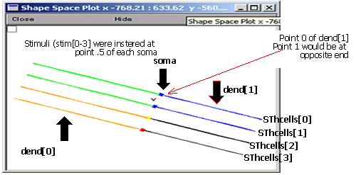
As you may be able to tell, there can be a lot of information to enter for each , particularly for complex al morphology where there are a large number of sections. To eliminate the need to enter this information in every .hoc file, and section positions may be randomly placed using built in random distributions, or the position data can be read from a file which may contain data from experimentally derived anatomical measurements. The diagram above is of 4 of our simple s which had a soma and 2 dendritc trees, one attached to the 0 end of the soma, the other attached to the 1 end. In each case the 0 side (proximal) of the dendrite is attached to the soma.
Using the code (SubThalNucl2.hoc) developed in the Connecting multiple s section C.2, this tutorial will show how to visualize the many s in the Graph>Shape plot window, how to manipulate voltage axis graphs and how to save a session (i.e. save the windows/variables so they can be opened again).
C.3.a 3D rotate objects in shape window
- Run the SubThalNucl2.hoc program.
- Open a shape graphs (Main Menu>>Graphs>>Shape Plot
- Right-click on the shape plot and release on "3D rotate"
- Use the left button to rotate the object by clicking and holding down the mouse button while moving the mouse across the window.
- To move the rotated object hold down the cntl key, hold down the left mouse button and move the mouse across the window.
C.3.b Graphing other aspects of the cell
C.3.c Moving text
C.3.d Deleting/removing certain variables
C.3.e The "View..." option
C.3.f Space plots
C.3.g Print and File Window Manager - saving a session
Space plots
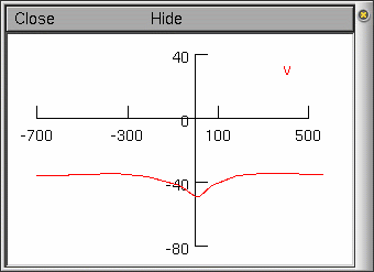
Time plots allow you to see exactly what happens to a variable vs. time at a single point in the . To see what happens at all points in a section (or a group of sections), you can use a space plot. Unfortunately, to generate a static graph of a variable vs. both time and space you need to produce a 3-D graph, gives you the next best thing: a movie-like graph called a space plot. This dynamic graph will plot a variable (e.g., voltage) vs. space for each time step in the simulation.
 To create
a space plot, select Shape plot from the Graph menu in the
Main Menu. This will open a shape plot window in which a schematic representation
of the will appear.
You can rotate the axes by selecting 3D Rotate from the Graph Properties menu. The middle mouse button is used to move the whole representation.
From this window, you can select from the menu (with the right mouse button) a Space Plot. By default, voltage is the variable to plot, but you can change this with the Plot What? menu item (e.g., to ina or m_hh). To create the space plot graph, you need to select a section of the to include in the space plot by clicking the left mouse button at the beginning of the section (in the schematic picture), dragging the mouse across the section you want to plot (while holding the mouse button down), and releasing the mouse button when you have covered the sections you want to plot. A line will appear from where you first clicked the mouse button to the current location of the pointer. When you release the mouse button, the sections you selected will be highlighted in colour, and a new window with the space plot will be opened. Press the Init & Run button in the RunControl window to see the space plot in action.

Acknowledgements
Last modified on 10/29/04 by
Albert Borroni, CS/Neuoriscience Oberlin College (aborroni@oberlin.edu)
based on tutorial written by
Andrew Gillies (andrew@anc.ed.ac.uk)
David Sterratt (dcs@anc.ed.ac.uk)
which is originally based on the tutorials by Kevin E. Martin
with the assistance of Ted Carnevale and Michael Hines